Distance Marching for Generative Modeling

Sampling trajectories of Distance Marching versus flow matching on a distance field over the data manifold — Middle row: outputs after 20% of the sampling steps. Ours, without time input, already shows the object. Flow matching, biased toward the data mean, is still noisy.

TL;DR

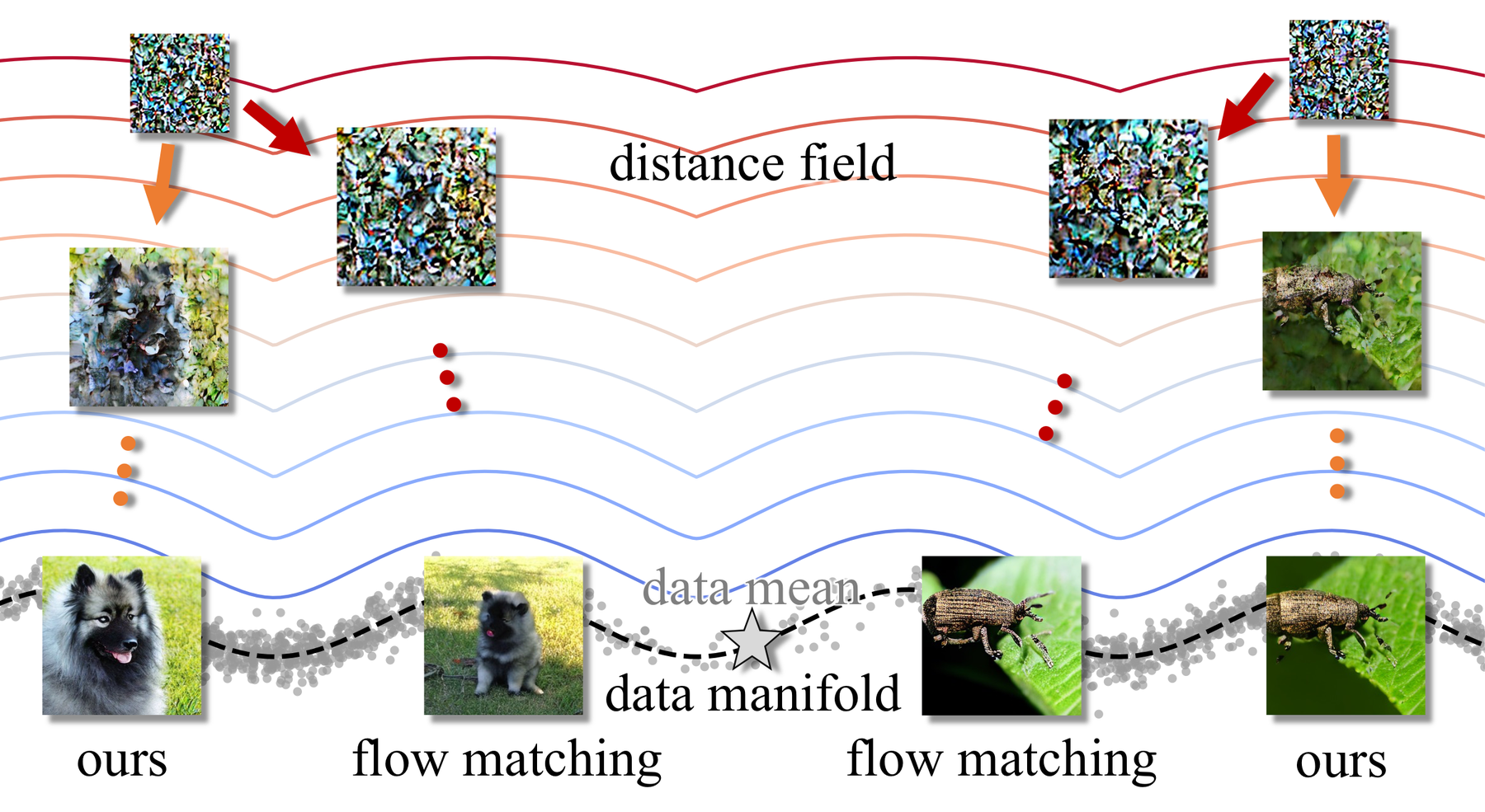
We model a distance field of the data manifold and generate by descending it, without time input. Our losses emphasize closer denoising targets. Among models without time input, ours is the only one that stays competitive with time-conditioned models across datasets and architectures.

Explore the trajectories

Sphere Tracing

Gradient Descent

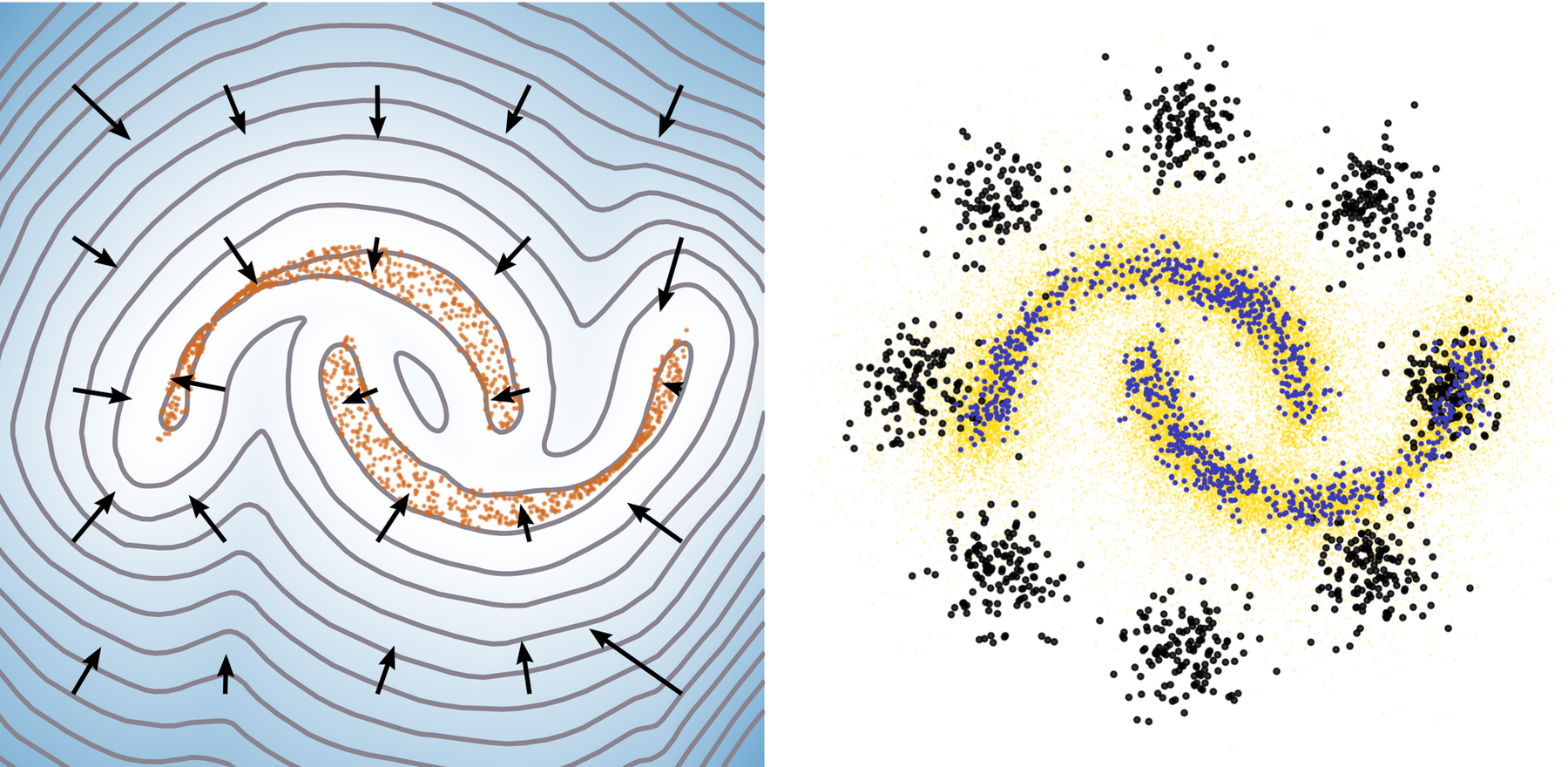
16 curated ImageNet 256×256 samples (XL/2, CFG 4.0, 250 steps). Each trajectory is projected onto its top three principal directions and shown with level sets of the predicted distance $u_\theta$.

Method

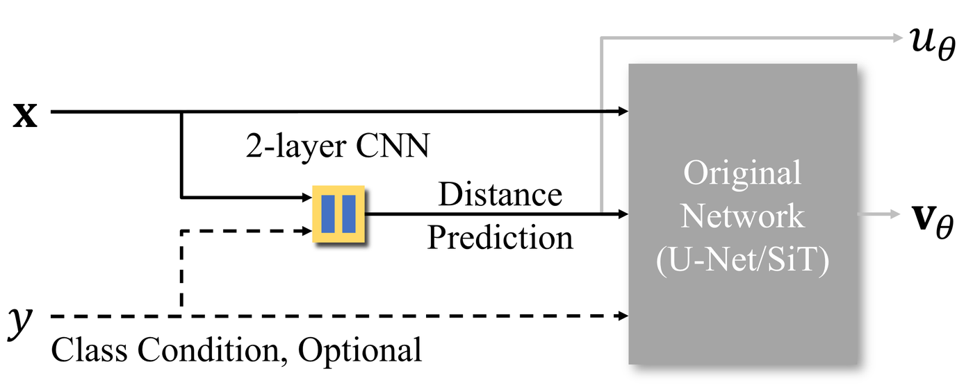
Architecture: a two-layer CNN head predicts the distance, which replaces the time embedding of the backbone

No time input: a two-layer CNN head predicts the distance $u_\theta(\mathbf{x})$ to the data manifold and feeds it to the unchanged backbone (U-Net or SiT) in place of the time embedding. The backbone predicts the denoising direction $\mathbf{v}_\theta(\mathbf{x})$. The head adds only 0.009%–0.19% parameters.

$\mathbf{x}$ linearly interpolates Gaussian noise and a data sample $\mathbf{s}$. We train with two losses:

One-Step Loss

$$\frac{\big\lVert \mathbf{x} - u_\theta(\mathbf{x})\,\mathbf{v}_\theta(\mathbf{x}) - \mathbf{s} \big\rVert^2}{\lVert \mathbf{x}-\mathbf{s}\rVert^2 + \epsilon}$$

Emphasizes closer data points and mitigates the bias toward the data mean.

Directional Eikonal Loss

$$\Big\lVert \mathbf{v}_\theta(\mathbf{x}) - \frac{\mathbf{x}-\mathbf{s}}{\sqrt{\lVert \mathbf{x}-\mathbf{s}\rVert^2 + c_0}} \Big\rVert^2$$

Constrains the direction of $\mathbf{v}_\theta$, which fixes the offset of the learned field to $c_0$.

From Gaussian noise, two deterministic samplers march toward the data manifold with step size $\eta$:

Sphere Tracing

$$\mathbf{x} \leftarrow \mathbf{x} - \eta\, u_\theta(\mathbf{x})\, \mathbf{v}_\theta(\mathbf{x})$$

Uses both the distance and the directional information.

Gradient Descent

$$\mathbf{x} \leftarrow \mathbf{x} - \eta\, \mathbf{v}_\theta(\mathbf{x})$$

Uses only the directional information.

Two moons: learned distance field and sphere-tracing trajectories — **Left:** two moons (orange) and the learned field $u_\theta$ with $-\nabla u_\theta$. **Right:** our samples: initial (black), intermediate (yellow), final (blue).

Results

CIFAR-10, unconditional

Method	w/o $t$	FID ↓
NCSN++		2.45
DDPM++		3.45
FM		6.35
EDM		1.99
1-RF FM		2.53
CLEL-large	✓	8.61
uEDM	✓	2.23
EM	✓	3.34
EqM	✓	3.36
Ours, gradient descent	✓	2.54
Ours, sphere tracing	✓	2.23

ImageNet 256×256, with CFG

Method	w/o $t$	FID ↓	IS ↑
SiT		7.66	254.77
uEDM	✓	7.96	–
EqM	✓	6.93	281.87
Ours, sphere tracing	✓	6.59	310.02
Ours, gradient descent	✓	6.67	311.31

Best over CFG scales per metric. B/2, 50k samples, 250 steps.

FID versus fraction of generation steps for SiT and our two samplers — We reach the final FID of flow matching (SiT, dopri5) in fewer than 60% of the steps. ImageNet, B/2, no CFG.

More sphere tracing samples on CIFAR-10

Sphere Tracing

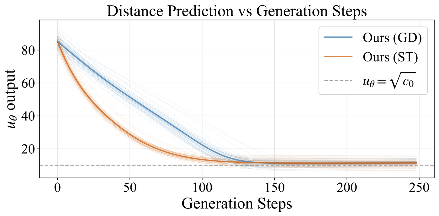
Using the predicted distance

Predicted distance over sampling steps on ImageNet — On ImageNet, $u_\theta$ settles near $\sqrt{c_0}$ before the 250 steps are used up.

Adaptive stopping

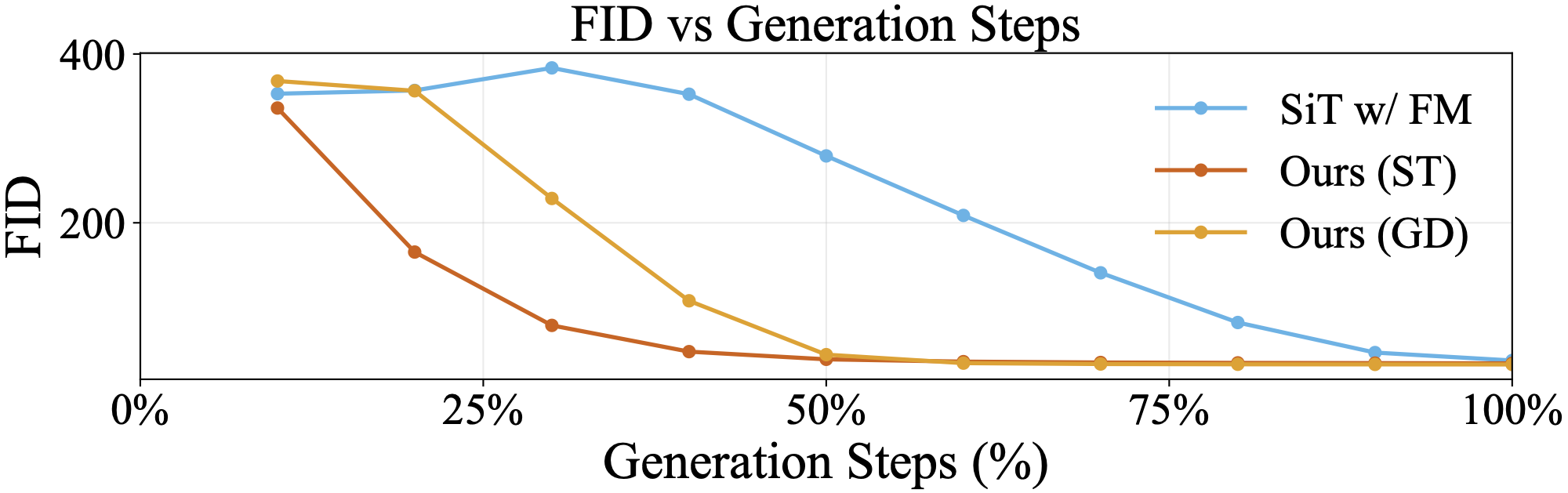
Stop gradient descent once $u_\theta$ rises for 10 consecutive steps: 29.7% fewer steps on ImageNet, better sFID and IS, slightly higher FID.

	Steps ↓	FID ↓	sFID ↓	IS ↑
Original gradient descent	250.0	32.16	7.52	45.16
Adaptive gradient descent	175.8	32.73	6.70	45.86

Out-of-distribution detection

Our 0.010M-parameter distance head gives the best average AUROC, with over 1000× fewer parameters than prior energy-based models.

	Params	SVHN	Textures	Constant	Avg.
PixelCNN++	54M	0.32	0.33	0.71	0.45
GLOW	44M	0.24	0.27	–	0.26
IGEBM	19M	0.63	0.48	0.39	0.50
EqM	130M	0.55	0.49	1.00	0.68
Ours	0.010M	0.94	0.49	0.95	0.79

AUROC ↑, CIFAR-10 in-distribution. Baselines from Yoon et al. (2023) and Wang & Du (2025).

BibTeX

@inproceedings{wang2026distancemarching,
  title     = {Distance Marching for Generative Modeling},
  author    = {Wang, Zimo and Mehta, Ishit and Lu, Haolin and Huang, Xunpeng and
               Sun, Chung-En and Yan, Ge and Weng, Tsui-Wei and Li, Tzu-Mao},
  booktitle = {Advances in Neural Information Processing Systems},
  year      = {2026}
}